LESSON 03 / 09 · MODELING & SIMULATION
Averaged Converter and LCL Plant
Where does an electrical oscillation come from?
THE CASE
Where does an electrical oscillation come from?
A small converter-voltage step creates a fast current oscillation before slower power control can react. An ideal current source cannot explain it. Retain the LCL plant and ask how energy moves through the circuit.
By the end of this lesson, you should be able to…
- Derive the LCL equations in a rotating frame.
- Separate physical inductance from virtual impedance.
03.01 MECHANISM & DERIVATION
Storage determines the electrical states
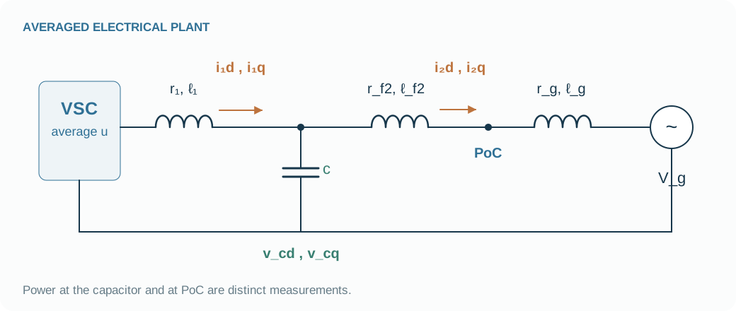
Each inductor current and capacitor voltage needs an evolution law. In dq coordinates, i₁, v_c and i₂ each contribute two components, giving six electrical states. The grid-side filter and grid inductance share i₂ and can be combined in series for the differential equation.
That simplification does not erase the PoC. Reconstruct its voltage across the filter branch when terminal measurements are needed. The open-loop lab steps average converter d-voltage by 0.005 pu at 10 ms; the 30 ms window and 2 μs integration step resolve the fast plant response.
03.02 MECHANISM & DERIVATION
Add the rotation terms with the right sign
Write KVL across each inductor and KCL at the capacitor, then differentiate in the rotating frame. With J = [[0, 1], [−1, 0]], every vector gains +ω_bωJ times itself. These cross-axis terms are coordinate effects; they do not create or consume energy.
Here ℓ = L/Z_b and c = CZ_b are time coefficients. Using nominal reactance in place of ℓ would change the derivative by a factor of ω_b. Keep the plant voltage u distinct from a controller power command: control must first generate u before these equations determine current.
\dot i_1=\frac{u-v_c-r_1i_1}{\ell_1}+\omega_b\omega Ji_1\dot v_c=\frac{i_1-i_2}{c}+\omega_b\omega Jv_c,\qquad\dot i_2=\frac{v_c-v_g-r_2i_2}{\ell_2}+\omega_b\omega Ji_2v_{PoC}=v_c-r_{f2}i_2-\ell_{f2}(\dot i_2-\omega_b\omega Ji_2)03.03 MECHANISM & DERIVATION
Initialize storage before evaluating the response
For this plant experiment, set i₂ = 0.6 + j0 at the infinite-bus port. Compute v_c = 1 + (r₂ + jω_bℓ₂)i₂, then i₁ = i₂ + jω_bcv_c and u = v_c + (r₁ + jω_bℓ₁)i₁. These values satisfy the steady circuit together.
Setting all currents to zero would instead simulate energization. Setting i₁ = i₂ would omit capacitor current. The distinction matters: this LCL case is initialized at the infinite-bus port, whereas the later reduced-model comparison matches power at PoC.
03.04 MECHANISM & DERIVATION
Use energy to audit the derivation
Define W = (ℓ₁|i₁|² + c|v_c|² + ℓ₂|i₂|²)/2. Differentiate it using the plant equations. Rotation terms cancel because a vector is orthogonal to its J rotation. What remains is input power minus bus export and resistive losses.
This identity checks several signs at once. A small energy-rate residual supports equation consistency; it does not validate neglected PWM or device limits. Closing the model with two power filters, one angle and four PI integrators produces the source 13-state droop realization.
\dot W=u^Ti_1-v_g^Ti_2-r_1\lVert i_1\rVert^2-r_2\lVert i_2\rVert^2FROM EQUATION TO JUDGMENT
Work the case
At nominal speed, let v_c = [1, 0] and c = 0.0008 s. Find the steady capacitor contribution to i₁q − i₂q.
- Set v̇_c = 0 in the capacitor equation.
- Since J[1,0] = [0,−1], the difference i₁ − i₂ is −ω_bcJv_c.
- The q component is +2π × 50 × 0.0008.
The contribution is +0.251327 pu. This fixed-voltage example illustrates why converter-side and grid-side current references differ.
FROM PREDICTION TO EVIDENCE
Watch the electrical time scale
A 0.005 pu d-voltage step at 10 ms excites the open-loop plant. Read i₂d and capacitor voltage together.
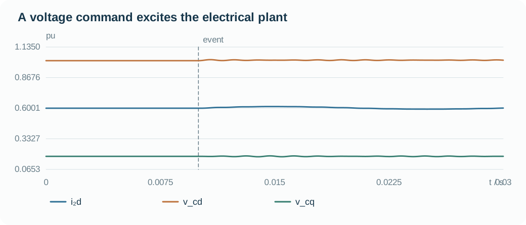
- The 10 ms converter-voltage step is the input; the inductor current follows through an evolution law.
- Capacitor voltage and output current respond together as energy moves between the stores.
- Use the energy-rate identity to check signs; the plotted oscillation alone cannot audit the equations.
Your experiment
- Run the +0.005 pu converter-voltage step and inspect the first 20 ms after the event.
- Reduce SCR from 5 to 2 and rerun; explain what changed in the electrical branch.
- Inspect lcl_run(): identify each stored-energy term and verify the energy-rate residual.
Laboratory · Python runs in your browser
Predict → run → inspect
Predict the response, then change a parameter and run. The initial plot is a baseline generated by the same solver. The first computation downloads Python; later runs reuse it.
Loading the baseline…
Numerical audit and samples
Six-state averaged LCL; open-loop voltage step at 10 ms, fixed 2 μs integration step. PI control, PWM, DC dynamics and current limits are omitted.
CHECK YOUR REASONING
Can you explain it—and calculate it?
Your engineering decision
Explain an observed oscillation through stored energy and coupling. Report the energy-rate residual alongside the current curve, then identify the inner loops needed to study damping under control.
REPRODUCE & EXTEND
Take the evidence into your model
Core equation reference
\dot i_1=\frac{u-v_c-r_1i_1}{\ell_1}+\omega_b\omega Ji_1\dot v_c=\frac{i_1-i_2}{c}+\omega_b\omega Jv_c,\qquad\dot i_2=\frac{v_c-v_g-r_2i_2}{\ell_2}+\omega_b\omega Ji_2v_{PoC}=v_c-r_{f2}i_2-\ell_{f2}(\dot i_2-\omega_b\omega Ji_2)\dot W=u^Ti_1-v_g^Ti_2-r_1\lVert i_1\rVert^2-r_2\lVert i_2\rVert^2Open the Python experiment and model source
The code reads the lab parameters and draws its own result. Edit the experiment or source to test your prediction. Download a single .py file with parameters, solver and experiment; local execution requires Python 3.
case is a snapshot of the controls when you press Run. Call solve(case) and assign the final solution to result to plot it.
The first run needs internet access to download Python. Computation stays in your browser; the solver uses only the standard library.
Ready to run.
Output appears here.
Python result
Inspect and edit the model source (advanced)
Source edits affect the next Python experiment; the lab above retains the original teaching equations.
Source materials and model scope
Based on local PINN-IBR materials reviewed on 2026-10-03. The website uses independent teaching realizations; low-frequency models retain nominal-frequency algebraic networks and ideal actuators. Continue into the detailed models below.
Coding/Modeling/src/ibrsim/models/droop_gfm.pyCoding/Modeling/src/ibrsim/conventions.py
WHAT FOLLOWS
We now know what receives the converter voltage. The next question is how a GFL controller acquires its reference angle and generates the current request.