LESSON 08 / 09 · MODELING & SIMULATION
Mode-Switching Hybrid Models
What must remain continuous when the controller changes?
THE CASE
What must remain continuous when the controller changes?
The inverter switches from GFL to VSM at 2 s, after a disturbance at 1 s. Both reduced state vectors have length four. Copying one vector into the other is tempting—and physically incorrect.
By the end of this lesson, you should be able to…
- Distinguish mode switching from parallel operation.
- Explain reset, hold, and release operations.
08.01 MECHANISM & DERIVATION
A mode changes the meaning of the active state
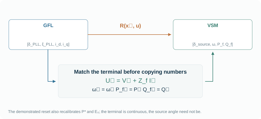
Between events, the active mode defines ẋ = f_m(x,u). At transition, a reset map defines x⁺ = R(x⁻,u). GFL uses [δ_PLL, ξ_PLL, i_d, i_q]; VSM uses [δ_source, ω, P_f, Q_f]. Equal dimension does not create compatible meaning.
A saved union of controller checkpoints is useful for implementation, but it is not automatically a larger ODE. Start the reset design from physical terminal quantities rather than array positions.
\dot x=f_m(x,u),\qquad x^+=R_{m^-\to m^+}(x^-,u)08.02 MECHANISM & DERIVATION
Reconstruct the incoming source from the terminal
Record V⁻, I⁻, P⁻, Q⁻ and PLL frequency just before switching. To preserve terminal current through Z_f, the incoming voltage source must be U⁺ = V⁻ + Z_fI⁻. Its source angle is arg U⁺, not necessarily the outgoing PLL angle.
Initialize VSM speed to the old estimated speed and its power filters to the measured powers. This aligns the incoming model with the outgoing terminal. The reset audit should then show terminal voltage, current, power and internal frequency jumps near roundoff.
U^+=V^-+Z_f I^-,\quad\delta^+=\arg U^+,\quad\omega^+=\omega^-,\quad P_f^+=P^-,\quad Q_f^+=Q^-08.03 MECHANISM & DERIVATION
Make the transition policy explicit
The teaching policy also chooses E₀⁺ to match source magnitude and P*⁺ = P⁻ + D(ω⁻ − 1) to make initial acceleration zero. It recalibrates the incoming command. Keeping the old command would be a different policy and could create an accelerating mismatch.
This experiment schedules one transition. A deployable design also needs guards, inactive-controller tracking, dwell rules, limits and protection. The source transition notebook treats hold/release policies and different active-state dimensions; a good endpoint response alone cannot establish a good transition.
E_0^+=|U^+|+n_q(Q^--Q^*),\qquad P^{*+}=P^-+D(\omega^--1)FROM EQUATION TO JUDGMENT
Work the case
For a fixed reset example, take V⁻ = 1 + j0, I⁻ = 0.6 + j0 and Z_f = 0.00625 + j0.1 pu. Find the incoming source angle.
- Multiply Z_fI⁻ = 0.00375 + j0.06.
- Add terminal voltage: U⁺ = 1.00375 + j0.06.
- Take atan2(0.06, 1.00375) and convert radians to degrees.
The incoming source angle is about 3.421°. The PLL can be voltage-aligned at 0° while the internal source requires a nonzero angle.
FROM PREDICTION TO EVIDENCE
Separate the disturbance from the reset
The disturbance is at 1 s; GFL-to-VSM switching is at 2 s. Read the terminal-compatible transition separately from the initial event.
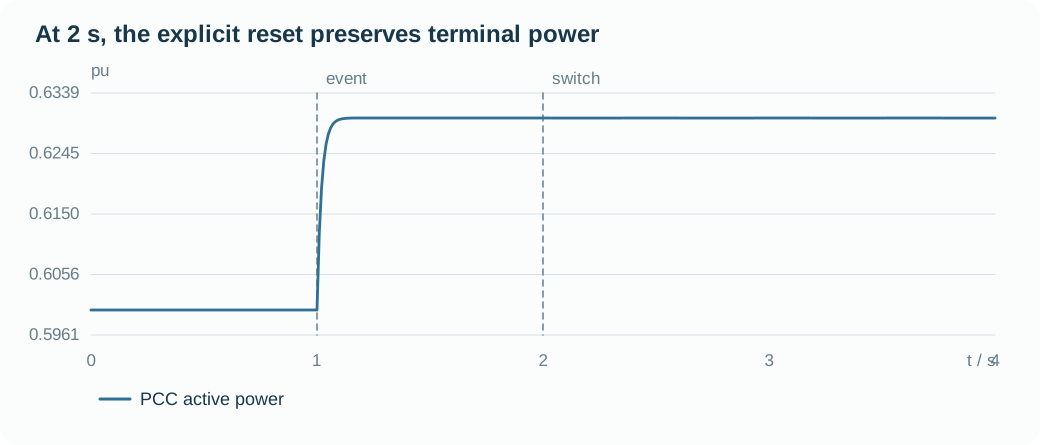
- The 1 s command disturbance and the 2 s mode transition are distinct events.
- At 2 s, the incoming source reconstructs the previous terminal using U⁺ = V⁻ + Z_fI⁻.
- Power continuity must be paired with voltage, current and frequency checks in the reset audit.
Your experiment
- Run the scheduled switch and inspect the trace immediately before and after 2 s.
- Read the reset residual and the final command offsets in the numerical audit.
- In reset_to_vsm(), deliberately replace the reset angle by the PLL angle; inspect the resulting jump.
Laboratory · Python runs in your browser
Predict → run → inspect
Predict the response, then change a parameter and run. The initial plot is a baseline generated by the same solver. The first computation downloads Python; later runs reuse it.
Loading the baseline…
Numerical audit and samples
Low-frequency teaching realization: nominal-frequency algebraic network and ideal current/voltage realization. 50 Hz, 10 kVA, 400 V; initial PCC total P = 0.6, Q = 0; X/R = 10. τᵢ = 0.02 s, τₚ = 0.1 s, τq = 0.05 s, nq = 0.0325; GFM source impedance 0.00625 + j0.1 pu. LCL, inner PI, DC dynamics and current limits are omitted.
CHECK YOUR REASONING
Can you explain it—and calculate it?
Your engineering decision
Write a continuity checklist and a command policy. Inspect the 2 s reset separately from the 1 s disturbance, then explain why angle equality is the wrong criterion here.
REPRODUCE & EXTEND
Take the evidence into your model
Core equation reference
\dot x=f_m(x,u),\qquad x^+=R_{m^-\to m^+}(x^-,u)U^+=V^-+Z_f I^-,\quad\delta^+=\arg U^+,\quad\omega^+=\omega^-,\quad P_f^+=P^-,\quad Q_f^+=Q^-E_0^+=|U^+|+n_q(Q^--Q^*),\qquad P^{*+}=P^-+D(\omega^--1)Open the Python experiment and model source
The code reads the lab parameters and draws its own result. Edit the experiment or source to test your prediction. Download a single .py file with parameters, solver and experiment; local execution requires Python 3.
case is a snapshot of the controls when you press Run. Call solve(case) and assign the final solution to result to plot it.
The first run needs internet access to download Python. Computation stays in your browser; the solver uses only the standard library.
Ready to run.
Output appears here.
Python result
Inspect and edit the model source (advanced)
Source edits affect the next Python experiment; the lab above retains the original teaching equations.
Source materials and model scope
Based on local PINN-IBR materials reviewed on 2026-10-03. The website uses independent teaching realizations; low-frequency models retain nominal-frequency algebraic networks and ideal actuators. Continue into the detailed models below.
Coding/Modeling/Single-IBR-Infinite-Bus/10_VSM_PLL_Transition_Infinite_Bus.ipynbCoding/Modeling/src/ibrsim/models/vsm_pll_transition.py
WHAT FOLLOWS
The final lesson puts all these interfaces into a reproducible comparison and turns curves into a defensible engineering recommendation.