Physics-informed GNN · Module 4
AI Preliminary · Neural Network Basics
The power-flow chapters gave us a way to compute operating points. Now ask a different question: can a trainable function learn an input–output relationship from examples? Before using a graph neural network to predict grid conditions, we need to understand what a neural network computes, what training changes, and what a small error does—and does not—tell us.
1. From physical computation to learning from data
Prerequisites: basic functions, matrix multiplication, derivatives, and the idea of a power-flow input and output. Prior machine-learning experience is not required. Start with the pictures and sliders; return to the batched gradient formulas after the worked example.
AI is the broad field; machine learning includes methods that learn patterns from data; deep learning uses neural networks with multiple representation layers. Here we study a modest one-hidden-layer multilayer perceptron (MLP) as the first neural-network building block. Training this model is numerical optimization, rather than a call to a conversational model.
- 1 · Physics & dataPower flow produces operating cases and voltage labels.
- 2 · Trainable functionUnpack an MLP using the small sin(x) example here.
- 3 · Train & validateOptimize parameters and evaluate data excluded from updates.
- 4 · Toward a GNNLater, encode buses, lines, and physical constraints explicitly.
Specify the task before choosing the network
In supervised regression, each example supplies an input x and a numerical target y. We choose a family of functions fθ and adjust its parameters θ using training examples. Predictions on new inputs are called inference. A classification task instead predicts a category; later, N-1 security could be formulated as classification or as regression of voltages, currents, or constraint margins.
For this chapter, the task is deliberately transparent:
The default has no noise; a slider adds Gaussian training-label noise. A line ŷ = ax + b can change its slope and offset, but cannot bend to follow the whole sine curve. This is a limitation of the chosen model class. A neural network adds nonlinear features; it still needs suitable data and successful optimization to fit well. A line would be entirely appropriate for a genuinely linear relationship.
2. A neuron is an affine map followed by an activation
The input weight w and hidden bias b position a feature; the output weight v and bias c combine it into a prediction. Parameters are numbers, not training examples. In this first experiment you set them; the training experiment later adjusts many such parameters automatically.
Lab A · Bend a curve by hand
Updates while dragging · no Python downloadHidden response and output
Calculation at the probe
w changes direction and steepness; b moves the activation region. v scales or flips the feature; c shifts the output vertically. The derivative gives the local slope at the probe.
Try w = −1, then return to w = 1 and vary b. Next set v = −1. What changes the input position of the bend, and what flips the output? With a linear activation, every slider combination still produces a line.
Why an activation is necessary
Without a nonlinear activation, stacking these affine layers collapses to one affine map. Nonlinearity changes the shapes the model can represent. This construction is explained further in Dive into Deep Learning: MLPs.
| Activation | Formula | Derivative | What to watch |
|---|---|---|---|
| tanh | tanh(z) | 1 − tanh²(z) | Smooth, signed response; small gradients when saturated |
| Sigmoid | 1 / (1 + exp(−z)) | σ(z)(1 − σ(z)) | Values between 0 and 1; also saturates |
| ReLU | max(0, z) | 1 for z > 0; 0 for z < 0 | Piecewise linear; code chooses derivative 0 at z = 0 |
| Linear | z | 1 | Control experiment: no nonlinear features |
These are hidden-layer choices. Our regression output remains linear so it can take positive and negative values. A sigmoid output is often used for a binary probability together with an appropriate classification loss; a hidden sigmoid by itself does not turn this regression into classification.
3. Many hidden features form an MLP
For a single input, H hidden units, and a single output:
Each hidden unit contributes w₂ⱼhⱼ, and the output adds these contributions and b₂. Training learns both the feature shapes and their combination. A large output weight alone does not establish importance: the feature value and the input range also matter. The lab selects three features by their RMS weighted contribution over the training interval, and includes all remaining terms as a fourth curve so their sum still equals the prediction.
Read matrix dimensions consistently
Use one observation per row, matching the NumPy code in the supplied Notebook. For N scalar inputs and H hidden units:
The vector of ones broadcasts a bias to every observation; H denotes width, while Hact denotes the activation matrix. There are H + H + H + 1 = 3H + 1 parameters: H = 16 gives 49, and H = 32 gives 97. In a column-vector convention, the transposes change; do not mix the two conventions inside a derivation.
4. Training: loss, gradients, and an update
The mean squared error (MSE) measures the average squared prediction error on the training examples:
η is the learning rate. Backpropagation computes the gradient by applying the chain rule through the computation graph; gradient descent then uses it to change the parameters. These are two separate steps. The full-batch experiment uses all training examples for each gradient and performs one update per epoch. A minibatch implementation would take several updates during one pass through its data.
- ① ForwardX → Z → H → Ŷ
- ② LossŶ, Y → L
- ③ BackwardL → ∇θL
- ④ Updateθ ← θ − η∇θL ↺
Worked example: one parameter gets one update
Take one observation x = 1, y = 0.8, with tanh, w = 1, b = 0, v = 0.5, c = 0. Its forward pass gives z = 1, h ≈ 0.761594, ŷ ≈ 0.380797, and L ≈ 0.175731. To update just w with η = 0.1:
The negative gradient increases w for this observation. If only w changes, the loss falls to approximately 0.172686. Full training computes gradients for all parameters using their old values, then updates them together. One successful step does not guarantee convergence of an entire nonconvex training problem.
Batched backpropagation, with shapes matching the forward pass
For tanh and scalar outputs, let D = ∂L/∂Ŷ. Sums below run over observations and preserve a row-shaped bias gradient.
The elementwise product combines the incoming gradient with each activation derivative. The standard-library Python source writes the same operations with scalar loops, so every factor remains visible. Frameworks such as PyTorch autograd compute graph derivatives automatically; automatic differentiation still needs a loss, data, and an optimizer.
Separate optimization from generalization
A very small learning rate may make slow progress; an excessive one can oscillate or diverge. A finite loss is not proof of convergence. Width changes representational capacity, while epochs and learning rate change optimization; failure to fit can come from either. More parameters do not automatically mean overfitting.
Training error measures examples used for updates. Validation helps choose settings on other examples; an untouched test set is reserved for final evaluation after those choices. Repeated tuning on a test set leaks information into development. See Google’s dataset-splitting explanation. The toy lab compares noisy training labels with the known clean target on distinct interpolation points, so the two errors measure different things when noise is enabled. It provides no final test-set claim.
5. Train a network and inspect what changed
First compare the default MLP with the best least-squares line. Replay epoch 0 and the last epoch. Then choose Linear activation: adding hidden units cannot rescue a model that is still affine. Finally try a learning rate of 1 to observe numerical failure and recover by lowering it.
Lab B · Train, compare, replay
Actual full-batch gradient descent · in your browserPreparing training…
Scrub after training. Curves, features, and metrics below follow the selected epoch. Python starts a full run using the settings above.
Target, samples, and current prediction
Loss through training (log₁₀ MSE axis)
How hidden units build the output
Settings retrain automatically; a fixed seed reproduces a run. Training points span [−π, π]; validation uses 160 distinct interior points with clean targets. Shaded regions show extrapolation outside the training interval and are excluded from validation metrics. There is no separate test set in this toy lab; it does not establish real-task generalization.
Use this controlled comparison: change one setting at a time, retain the seed, compare losses at the same epoch, and inspect the curve. Increasing width can improve a fit, but an insufficient optimization budget can hide that capacity. Adding noise and reducing the sample count makes the distinction between fitting observations and recovering a clean function visible; a particular run need not exhibit overfitting.
6. Run and modify the Python implementation
The JavaScript lab runs the explicit equations quickly. This panel executes the Python implementation of the same algorithm, with matched initialization, random sampling, and update order. The original NumPy teaching Notebook remains available below; the new self-contained Notebook uses this readable standard-library model and Matplotlib for figures. No pretrained network or hidden training service is involved.
1 · Inspect the input case
A run copies Lab B's target, activation, width, sample count, noise, learning rate, epoch count, and seed. This snapshot follows those controls; replay only inspects saved parameters and does not change case.
2 · Expand model source and dependencies (editable)
Only the Python standard-library math module is required. dataset() creates data; initialize() creates parameters; predict() is the forward pass; gradient() applies the chain rule; step() updates weights; train() assembles the workflow and returns curves and metrics. Source edits apply to the next Python run.
3 · What does main() do?
Copy the settings, call train(parameters) to generate data, initialize, optimize, and validate, then print metrics and return answer. The final result = main() passes that return value to the plot. Editing parameters here does not change the sliders.
The first run downloads Pyodide. Training runs in a browser worker without an account or API key. The standard-library version prioritizes readability and can be slower than the JavaScript lab for large settings. You can stop a run; a reload clears code edits that have not been downloaded.
Ready to run.
Output appears here.
Prediction returned by Python (separate from replay)
Try uncommenting parameters["hidden"] = 32, or set parameters["target"] = "sin2". To change the algorithm, expand model.py and inspect gradient() before modifying it. A useful verification is a central finite difference of the loss: it should agree with an analytic gradient away from ReLU’s kink. The downloadable Notebook includes this check.
7. From an MLP to a power-system learning task
Return to the preceding pandapower chapter. Each supplied, converged operating case can provide inputs and labels: load/generation settings and topology in; voltages, currents, or security margins out. An islanded or nonconverged solve must carry a separate status rather than become a fabricated zero-voltage training label.
A useful project workflow is to define the label and security criterion, generate and audit cases, split scenarios before fitting preprocessing, train a baseline, and evaluate on held-out conditions. Keep closely related cases and their contingencies grouped to prevent leakage. Voltage and current limits, unsupplied buses, and convergence status need explicit treatment. A small average voltage error alone does not establish accurate N-1 security classification.
| Architecture | Structural idea | Power-system connection |
|---|---|---|
| MLP | Dense transformations of a fixed vector | A baseline for a fixed bus ordering and topology representation |
| CNN | Shared local filters on a grid | Spatially arranged signals or grid-like measurements |
| RNN / LSTM / GRU | A hidden state carried through a sequence | Temporal measurements and forecasting |
| Transformer | Attention between represented elements | Context across sequences or sets, with suitable position/structure information |
| GNN | Messages along graph connections | Bus features, line features, and changing network connectivity |
| Autoencoder / VAE | Encode and reconstruct, optionally with a probabilistic latent model | Representation learning and anomaly detection |
| GAN / diffusion | Different objectives for learning generative distributions | Synthetic scenarios; generated samples still need physical checks |
A graph-aware architecture is a useful structural choice; it does not automatically enforce Kirchhoff’s laws or guarantee transfer to every topology. A later physics-informed objective may combine a data-fit term with a precisely defined AC residual and constraint terms. The variables, sign conventions, normalization, and relative weighting of those terms must be stated. This chapter trains only a supervised MLP.
Extension from the supplied slides: Neural ODE and GFM models
The original slides place neural networks between dynamical-model lessons and Neural ODEs. The same function-approximation idea can parameterize a state derivative, ds/dt = fθ(s, u), with an ODE solver constructing the trajectory. This changes the meaning of the output and the training problem. It is a different use from a static power-flow surrogate; fitting sine here does not identify a GFM dynamic model. See the separate IBR dynamics curriculum for that learning path.
8. Practice: predict, run, explain
- With no nonlinear activation, increase width from 2 to 32. Explain why the model still cannot reproduce the entire sine curve.
- Keep the default seed and width. Compare η = 0.001, 0.03, and 1 at the same epoch budget. Distinguish slow optimization from numerical divergence.
- Switch to sin(2x). Compare widths 4, 16, and 32, and justify whether changing the epoch budget changes your conclusion.
- Use 16 training points and noise 0.3. Compare train and validation errors carefully: what differs about their targets? Inspect the shaded extrapolation region separately.
- At a chosen replay frame, add the three feature curves and the remaining-terms curve at one x. Why must the result equal the MLP output?
- Draft a power-grid dataset schema with inputs, labels, units, topology/status fields, split groups, and the chosen N-1 security criterion. Identify a potential leakage path.
Checkpoint: can you explain the complete experiment?
The model family determines possible shapes. The loss defines the training objective. Backpropagation computes derivatives; the optimizer updates parameters. Validation checks excluded examples during development. A final evaluation needs an appropriate untouched test set and the actual physical task’s metrics. Neither fitting a sine curve nor reducing training MSE proves power-system security performance.
9. Slides, notebooks, and further reading
This webpage reorganizes the supplied 33-slide Neural Network Basics deck and its 22-cell teaching Notebook as module 4 of this course. Their “Week 4 / next week” references belong to the original dynamics teaching sequence. The downloads preserve that context; the webpage adds the GNN transition, parameter experiments, explicit row-vector notation, and validation/extrapolation distinctions.
Architecture overview from the supplied materials
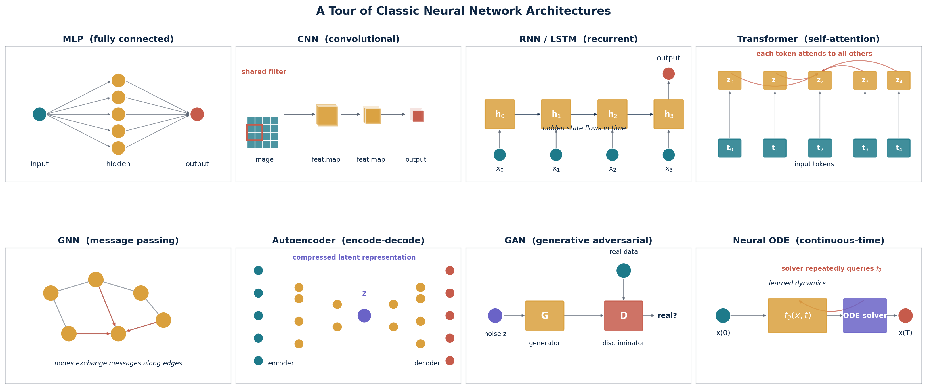
Further reading: D2L: MLPs and activations, PyTorch: automatic differentiation, and Google ML Crash Course: training, validation, and test sets.