L01 / Course & power-system overview
Course Orientation & Logistics
People, course expectations, tools, assessments, and the power-system design workflow.
01 / UNDERSTAND & PREDICT
Understand the model, then predict the result
Follow the original explanations, diagrams, derivations, and examples in slide order, then use the companion experiment below.
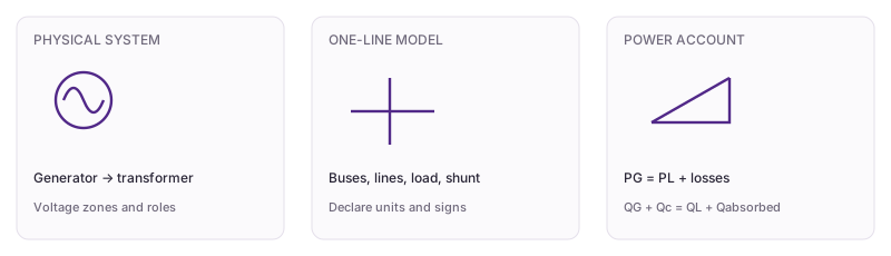
- Explain generators, transformers, lines, buses, loads, and shunt compensation.
- Distinguish MW, Mvar, and MVA and reconcile power with a declared sign convention.
- Declare data, reference directions, and assumptions before interpreting a result.
Working through the course
Estimate orders of magnitude by hand, reproduce them in editable Python, then check units, signs, balances, and limits. Slides, the textbook, Python, and PowerWorld support the course; these web experiments explain steady-state models.
Baseline example: check each step
- Receiving bus: Qnet = 30 − 10 = 20 Mvar.
- Line sending end: P = 83 MW and Q = 25 Mvar.
- Generator: P = 84 MW and Q = 27 Mvar.
- Using 138 kV line voltage and sending-end |S| gives balanced current ≈ 362.657 A.
Cross-check the original slides
02 / EXPLORE
Change one input and explain the response
Compare current at 69 and 138 kV. Explain why physical I²R losses require a line-impedance model.
Advanced parameters / test readings
Preparing the model.
Power at the declared boundaries
Current intermediate values and numerical checks
This account uses prescribed equipment losses and a balanced three-phase current estimate. Voltage changes the estimated current; loss values remain input data.
03 / EDIT & COMPUTE
Edit code to reproduce the model independently
Reproduce the baseline, then modify the parameter scan. The source contains reusable independent model functions; edit the current function and inspect numerical checks.
case is a snapshot of the controls when you press Run. Call solve(case) and assign the final solution to result to plot it.
The first run needs internet access to download Python. Computation stays in your browser; the solver uses only the standard library.
Ready to run.
Output appears here.
Last Python run and current control reference
Inspect and edit the model source (advanced)
Edit this module's function and run again. case.module selects the module; solve(case) returns values, plots, and checks. The parameter experiment keeps the original JavaScript reference for comparison.
04 / CHECK & EXPLAIN
Companion experiment practice and feedback
Load 80 MW/30 Mvar; capacitor 10 Mvar; line loss 3 MW/absorption 5 Mvar; transformer loss 1 MW/absorption 2 Mvar.
Practice uses fixed baseline inputs independently of the controls. Each field displays its tolerance.
See the worked solution
- Receiving bus: Qnet = 30 − 10 = 20 Mvar.
- Line sending end: P = 83 MW and Q = 25 Mvar.
- Generator: P = 84 MW and Q = 27 Mvar.
- Using 138 kV line voltage and sending-end |S| gives balanced current ≈ 362.657 A.
Finally, explain in your own words
- What are the inputs, references, and main assumptions?
- Compare current at 69 and 138 kV. Explain why physical I²R losses require a line-impedance model.
- Did your code edit change physical parameters, the method, or representation bases? Which check helps identify that?
Passing numerical and understanding checks records this lecture’s companion practice as “practice checks passed.”