L13 / Per-unit systems
Per Unit System I
Choose coherent bases and normalize voltage, current, impedance, admittance, and power.
01 / UNDERSTAND & PREDICT
Understand the model, then predict the result
Follow the original explanations, diagrams, derivations, and examples in slide order, then use the companion experiment below.
- Choose power and voltage bases before deriving current and impedance bases.
- Distinguish single-phase terminal bases from three-phase line-voltage/total-power bases.
- Verify invariant per-unit impedance on corresponding transformer bases.
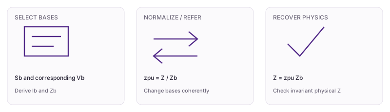
Independent and derived bases
After choosing Sb and Vb, derive other bases coherently. Three-phase uses total Sb and line voltage Vb,LL; single-phase uses terminal voltage and single-phase Sb.
Normalize and recover
Divide physical quantities by matching bases, then multiply back to recover them. Coherent voltage, current, and power bases give |Spu|=Vpu Ipu in three-phase.
Baseline example: check each step
- For three-phase Sb=100 MVA, Vb,H=138 kV and a=10, Vb,L=13.8 kV.
- Zb,L=1.9044 Ω and Ib,L≈4183.698 A.
- 1+j4 Ω gives zpu≈0.525100+j2.100399.
- Referring to HV gives 100+j400 Ω with Zb,H=190.44 Ω and the same zpu.
- Halving the power base at fixed voltage bases halves zpu, while recovery with the new Zb retains physical Z.
Cross-check the original slides
02 / EXPLORE
Change one input and explain the response
Change only Sb and check physical recovery. Change Vb,H and inspect the square dependence. Edit the Python base formula and use recovery error to test it.
Advanced parameters / test readings
Preparing the model.
Base changes and per-unit impedance
Recovery of the same physical impedance
Current intermediate values and numerical checks
This lab uses corresponding voltage ratios, one power base, and a fixed physical impedance. Switching single/three-phase changes quantity interpretation; labels state voltage and total-power conventions.
03 / EDIT & COMPUTE
Edit code to reproduce the model independently
Reproduce the baseline, then modify the parameter scan. The source contains reusable independent model functions; edit the current function and inspect numerical checks.
case is a snapshot of the controls when you press Run. Call solve(case) and assign the final solution to result to plot it.
The first run needs internet access to download Python. Computation stays in your browser; the solver uses only the standard library.
Ready to run.
Output appears here.
Last Python run and current control reference
Inspect and edit the model source (advanced)
Edit this module's function and run again. case.module selects the module; solve(case) returns values, plots, and checks. The parameter experiment keeps the original JavaScript reference for comparison.
04 / CHECK & EXPLAIN
Companion experiment practice and feedback
Three-phase Sb=100 MVA, Vb,H=138 kV, a=10, physical LV Z=1+j4 Ω.
Practice uses fixed baseline inputs independently of the controls. Each field displays its tolerance.
See the worked solution
- For three-phase Sb=100 MVA, Vb,H=138 kV and a=10, Vb,L=13.8 kV.
- Zb,L=1.9044 Ω and Ib,L≈4183.698 A.
- 1+j4 Ω gives zpu≈0.525100+j2.100399.
- Referring to HV gives 100+j400 Ω with Zb,H=190.44 Ω and the same zpu.
- Halving the power base at fixed voltage bases halves zpu, while recovery with the new Zb retains physical Z.
Finally, explain in your own words
- What are the inputs, references, and main assumptions?
- Change only Sb and check physical recovery. Change Vb,H and inspect the square dependence. Edit the Python base formula and use recovery error to test it.
- Did your code edit change physical parameters, the method, or representation bases? Which check helps identify that?
Passing numerical and understanding checks records this lecture’s companion practice as “practice checks passed.”