L12 / Transformer modeling
Transformer Modeling III
Infer transformer parameters from open- and short-circuit tests; calculate regulation and efficiency.
01 / UNDERSTAND & PREDICT
Understand the model, then predict the result
Follow the original explanations, diagrams, derivations, and examples in slide order, then use the companion experiment below.
- Distinguish winding turns ratio from three-phase line-voltage ratio.
- Infer equivalent parameters from open/short tests with consistent referred sides.
- Estimate regulation, copper loss, and efficiency and check approximation conditions.
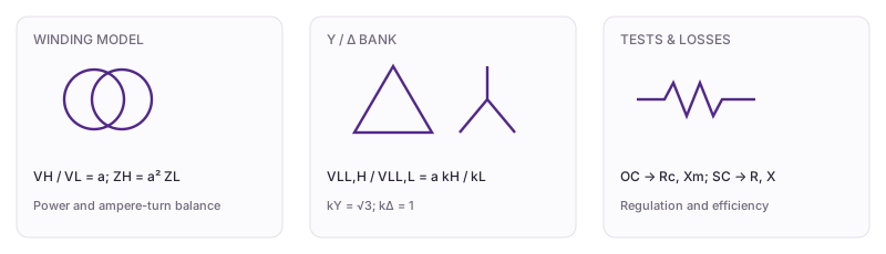
Open- and short-circuit tests
The open test identifies excitation: Ic=Poc/Voc and Im=√(Ioc²−Ic²). The short test identifies series terms: |Zeq|=Vsc/Isc and Req=Psc/Isc². Readings require P≤VI and parameters need their test side.
Nonideal model and approximations
Resistance gives copper loss, leakage reactance gives series drop, and excitation represents magnetization and core loss. Here rated-base rpu, xpu and loading λ estimate regulation at lagging pf.
Power and efficiency
Real output is Srated×λ×pf. Copper loss varies with λ² and core loss is approximately constant at fixed voltage. Check ideal bank ratios separately from loss-based efficiency.
Baseline example: check each step
- Bank teaching case: 138 kV, a=10, Y–Y, 30 MVA, loading 0.8, pf=0.9.
- No-load LV line voltage is 13.8 kV; ideal LV line current ≈ 1004.087 A.
- rpu=0.01 and xpu=0.08 give ≈ 3.510% regulation; copper and 30 kW core loss give ≈ 98.983% efficiency.
- The independent L12 test case is a 10 kVA, 2400/240 V single-phase unit. OC gives Rc,L=480 Ω and Xm,L≈123.935 Ω.
- SC gives Req,H≈10.368 Ω and Xeq,H≈26.869 Ω. Refer excitation parameters to HV using the test transformer’s fixed ratio 10².
Cross-check the original slides
- L10 · Transformer Modeling I
- L11 · Transformer Modeling II
- L12 · Transformer Modeling III
- L20 · Three-Phase Transformers I (post-Exam-1 extension)
- L21 · Three-Phase Transformers II (post-Exam-1 extension)
02 / EXPLORE
Change one input and explain the response
Switch to Δ–Y and check line ratio a/√3. Raise OC watts above VI and inspect the consistency feedback; explain why invalid readings cannot determine parameters.
Advanced parameters / test readings
Preparing the model.
Approximate regulation versus loading
Efficiency versus loading
Current intermediate values and numerical checks
The bank uses ideal winding magnitudes and first-order small-drop approximations. L12 tests concern a separate fixed 10 kVA single-phase unit; they do not parameterize this bank. L20–L21 are the post-Exam-1 connection extension.
03 / EDIT & COMPUTE
Edit code to reproduce the model independently
Reproduce the baseline, then modify the parameter scan. The source contains reusable independent model functions; edit the current function and inspect numerical checks.
case is a snapshot of the controls when you press Run. Call solve(case) and assign the final solution to result to plot it.
The first run needs internet access to download Python. Computation stays in your browser; the solver uses only the standard library.
Ready to run.
Output appears here.
Last Python run and current control reference
Inspect and edit the model source (advanced)
Edit this module's function and run again. case.module selects the module; solve(case) returns values, plots, and checks. The parameter experiment keeps the original JavaScript reference for comparison.
04 / CHECK & EXPLAIN
Companion experiment practice and feedback
Bank: VH,LL=138 kV, a=10, Y–Y. Independent L12 test unit: 10 kVA, 2400/240 V; OC(LV) 240 V/2 A/120 W; SC(HV) 120 V/4.1667 A/180 W.
Practice uses fixed baseline inputs independently of the controls. Each field displays its tolerance.
See the worked solution
- Bank teaching case: 138 kV, a=10, Y–Y, 30 MVA, loading 0.8, pf=0.9.
- No-load LV line voltage is 13.8 kV; ideal LV line current ≈ 1004.087 A.
- rpu=0.01 and xpu=0.08 give ≈ 3.510% regulation; copper and 30 kW core loss give ≈ 98.983% efficiency.
- The independent L12 test case is a 10 kVA, 2400/240 V single-phase unit. OC gives Rc,L=480 Ω and Xm,L≈123.935 Ω.
- SC gives Req,H≈10.368 Ω and Xeq,H≈26.869 Ω. Refer excitation parameters to HV using the test transformer’s fixed ratio 10².
Finally, explain in your own words
- What are the inputs, references, and main assumptions?
- Switch to Δ–Y and check line ratio a/√3. Raise OC watts above VI and inspect the consistency feedback; explain why invalid readings cannot determine parameters.
- Did your code edit change physical parameters, the method, or representation bases? Which check helps identify that?
Passing numerical and understanding checks records this lecture’s companion practice as “practice checks passed.”