L05 / Single-phase AC circuits
Single-Phase AC Circuits I
Map sinusoidal waveforms to RMS phasors; convert and add polar and rectangular representations.
Follow the original explanations, diagrams, derivations, and examples in slide order, then use the companion experiment below.
01 / UNDERSTAND
From one waveform to one phasor
Why can the same voltage be described as both 120 V and 169.7 V? Start with the slide deck's opening question.
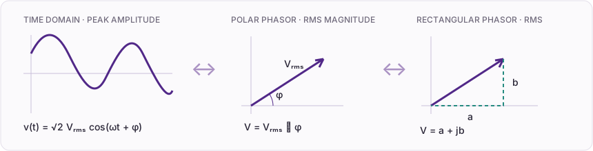
By the end, distinguish peak from RMS, convert a sinusoid to polar and rectangular phasors, identify lead/lag, and add compatible voltage phasors before reconstructing the waveform.
1. Declare references and units
Use a cosine reference, RMS phasors, and degree inputs. Convert phase angles to radians in calculation. Angular frequency ω is in rad/s; f is in Hz; T = 1/f.
2. Understand RMS
With cos²θ = (1 + cos2θ)/2, the oscillating term averages to zero over a period. A sinusoid therefore has V̂ = √2 Vᵣₘₛ. RMS gives the DC voltage producing the same average heating in the same resistor.
3. Choose the calculation form
For addition, add real and imaginary parts separately. Recover magnitude with √(a² + b²) and angle with atan2(b, a) to retain the quadrant. Magnitudes add directly only when the two phasors align.
4. Identify lead and lag
At the same frequency, voltage at +30° leads current at −20° by 50°. Positive phase shifts a waveform left of the zero-phase cosine. Use the principal difference from −180° to 180°; a 180° separation is opposition without a unique lead/lag direction.
Slide example CE-2A: convert → add → reconstruct
Given vₛ(t) above, i(t) = 10√2 cos(377t − 20°) A, and Vₓ = 40∠−60° V, follow the slide sequence. Displayed results use three decimals; calculations retain full precision.
- Use RMS and retain phaseVₛ = 120∠30° V; I = 10∠−20° A; φV − φI = 50°.
- Convert to rectangular formVₛ = 103.923 + j60.000 V; Vₓ = 20.000 − j34.641 V.
- Add matching componentsVₜ = 123.923 + j25.359 V = 126.491∠11.565° V.
- Reconstruct and checkvₜ(t) = 126.491√2 cos(377t + 11.565°) V; V̂ₜ = 178.885 V.
The slides use ω = 377 rad/s, giving f ≈ 60.001 Hz, displayed as 60.0 Hz. The experiment retains 377 rather than replacing it with a rounded frequency.
02 / PREDICT & EXPLORE
Make the phasors and waveforms move together
Predict first: if Vₓ aligns with Vₛ, will the resultant RMS be 120 + 40? If equal magnitudes oppose, is the resultant angle still defined? Then test your prediction.
Preparing the experiment.
RMS phasors: head-to-tail addition
Time domain: same-frequency voltage sum
Current calculation: components → phasor → waveform
Compare voltage and current by phase
Each curve is divided by its own peak to compare phase only; they do not share physical units or amplitudes. Current RMS remains 10 A.
- Change only ω. How does the time scale change? Do phasor magnitudes or angles change?
- Move Vₓ from −60° to +30°. Explain why the magnitude changes instead of always equaling the sum of magnitudes.
- Select Cancellation. Inspect voltage, RMS, and angle, and explain why a zero vector has no direction.
03 / EDIT & COMPUTE
Edit Python to reproduce and test the result
The code receives the slider inputs. Run the baseline to check the waveform and RMS, then edit a phase or the model. Code results are plotted separately against the current reference.
case is a snapshot of the controls when you press Run. Call solve(case) and assign the final solution to result to plot it.
The first run needs internet access to download Python. Computation stays in your browser; the solver uses only the standard library.
Ready to run.
Output appears here.
Student code and reference: resultant voltage
Inspect and edit the model source (advanced)
The phasor conversion, complex addition, and waveform reconstruction functions execute on the next run. Edit the calculation and compare numerically integrated RMS with phasor magnitude. The parameter experiment retains the original reference model.
solve(case), add case["vx_angle_deg"] = case["vs_angle_deg"]. Predict the RMS, then run it. Next load the phase sweep from −180° to 180° and explain its maximum and minimum magnitudes.Differences may come from edited inputs or calculations. Check the case before interpreting every difference as an error.
04 / CHECK & EXPLAIN
Solve slide practice CE-2D independently
Find V꜀ = Vₐ + Vᵦ and v꜀(t). This exercise uses the fixed inputs above, independent of the sliders. Find rectangular components, then RMS, angle, and peak.
Voltage tolerance: ±0.05 V; angle tolerance: ±0.05°. Angles are compared modulo 360°.
See the worked solution
Vₐ = 72.505 − j33.809 V; Vᵦ = 20.521 − j56.382 V.
V꜀ = 93.026 − j90.191 V = 129.569∠−44.114° V.
v꜀(t) = 129.569√2 cos(377t − 44.114°) V; V̂꜀ ≈ 183.239 V.
Positive real and negative imaginary components place the resultant in quadrant IV. Reversing the polar conversion should reproduce both components.
Explain in your own words
- Why does a phasor use RMS, while waveform reconstruction needs √2?
- Why does changing ω leave the phasor result unchanged but change the waveform's time scale?
- Did your Python edit change the inputs, representation, or physical model? How can you check?
L06 connects these voltage and current phasors to real, reactive, and complex power.
Source:L05_single_phase_ac_i/L05_single_phase_ac_i.pdf · Opening problem, CE-2A, and CE-2D follow the current slides. Web diagrams and experiments are course-authored. The model covers sinusoidal quantities at a shared frequency.