L07 / Single-phase AC circuits
Single-Phase AC Circuits III
Determine target reactive power, shunt compensation, and capacitance for power-factor correction.
01 / UNDERSTAND & PREDICT
Understand the model, then predict the result
Follow the original explanations, diagrams, derivations, and examples in slide order, then use the companion experiment below.
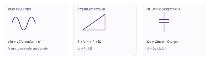
- Keep RMS, cosine reference, and current direction consistent.
- Use the current conjugate to calculate P, Q, |S|, and power factor.
- Calculate target Q, capacitor rating, and corrected source current.
Conjugate and signs
Current enters the positive load terminal, using the passive convention. Δφ = φV−φI; positive Δφ means lagging current and positive Q. Calculate S = V I* before reading P and Q.
Shunt correction
Keep load P fixed. Target lagging Q is P tan(arccos target pf), and Qc = Qload−Qtarget. Add capacitance only to reduce inductive Q; this lab adds none when the target is already met or the load is capacitive.
Baseline example: check each step
- Δφ = 50° and |S| = 1200 VA.
- P ≈ 771.345 W, Q ≈ 919.253 var, pf ≈ 0.643 lagging.
- Target Q ≈ 253.529 var; capacitor rating ≈ 665.724 var.
- C ≈ 122.628 μF; load current remains 10 A while source current falls to ≈ 6.766 A.
Cross-check the original slides
02 / EXPLORE
Change one input and explain the response
Set Δφ to −30° and explain Q and the absence of added capacitance. Edit the Python phase and check P²+Q²=|S|².
Advanced parameters / test readings
Preparing the model.
Voltage/current phase comparison
Instantaneous and average power
Current intermediate values and numerical checks
The model assumes single-frequency sinusoidal steady state, fixed voltage, and fixed load power. Correction changes source Q and current; normalized curves compare phase only.
03 / EDIT & COMPUTE
Edit code to reproduce the model independently
Reproduce the baseline, then modify the parameter scan. The source contains reusable independent model functions; edit the current function and inspect numerical checks.
case is a snapshot of the controls when you press Run. Call solve(case) and assign the final solution to result to plot it.
The first run needs internet access to download Python. Computation stays in your browser; the solver uses only the standard library.
Ready to run.
Output appears here.
Last Python run and current control reference
Inspect and edit the model source (advanced)
Edit this module's function and run again. case.module selects the module; solve(case) returns values, plots, and checks. The parameter experiment keeps the original JavaScript reference for comparison.
04 / CHECK & EXPLAIN
Companion experiment practice and feedback
V=120 V RMS, I=10 A RMS, voltage leads current by 50°, ω=377 rad/s, target pf=0.95 lagging.
Practice uses fixed baseline inputs independently of the controls. Each field displays its tolerance.
See the worked solution
- Δφ = 50° and |S| = 1200 VA.
- P ≈ 771.345 W, Q ≈ 919.253 var, pf ≈ 0.643 lagging.
- Target Q ≈ 253.529 var; capacitor rating ≈ 665.724 var.
- C ≈ 122.628 μF; load current remains 10 A while source current falls to ≈ 6.766 A.
Finally, explain in your own words
- What are the inputs, references, and main assumptions?
- Set Δφ to −30° and explain Q and the absence of added capacitance. Edit the Python phase and check P²+Q²=|S|².
- Did your code edit change physical parameters, the method, or representation bases? Which check helps identify that?
Passing numerical and understanding checks records this lecture’s companion practice as “practice checks passed.”