L03 / Generation mix planning
Optimal Fuel Mix Analysis I
Demand, energy, capacity factor, planning reserve margin, and load-duration curves.
01 / UNDERSTAND & PREDICT
Understand the model, then predict the result
Follow the original explanations, diagrams, derivations, and examples in slide order, then use the companion experiment below.
- Sort a load record and verify unchanged energy.
- Calculate reserve capacity targets and GT/CC crossover hours.
- Cover net load, then check accredited reserve and identify the simplifications.
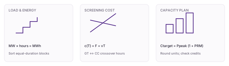
Power, energy, and capacity
Demand in MW is a rate. A two-hour block contributes MW×2 h to MWh. The L03 daily record and L04 annual record are distinct; do not treat one day as a year.
Duration curves and reserve
Sorting equal-duration blocks retains energy but loses chronology. Compare reserve with accredited planning capacity; that check alone does not establish reliability at every operating time.
Baseline example: check each step
- L03: twelve two-hour blocks total 77960 MWh; peak is 4380 MW.
- Current PRM ≈ 10.731%; the 15% target is 5037 MW, leaving 187 MW.
- GT/CC crossover is ≈ 4511.481 h/year; GT costs less at 2000 h.
- The simplified L04 net load assigns 1800 MW to CC; rounding to four CC units leaves six GT units for peak coverage.
- Default renewable capacity credit is zero; seven additional GT units give 4915 MW ≥ the 4830 MW reserve target.
Cross-check the original slides
02 / EXPLORE
Change one input and explain the response
Set equal GT and CC variable costs and inspect the lack of a unique crossover. Change capacity credit and explain why energy output and reserve credit are separate inputs.
Advanced parameters / test readings
Preparing the model.
L03: chronological and sorted load
L04: annual screening costs
Current intermediate values and numerical checks
Renewable output blocks are constant and capacity credit is a separate input. Rounding and adding GT give a feasible teaching portfolio; costs use fixed/variable coefficients without startup or ramp constraints.
03 / EDIT & COMPUTE
Edit code to reproduce the model independently
Reproduce the baseline, then modify the parameter scan. The source contains reusable independent model functions; edit the current function and inspect numerical checks.
case is a snapshot of the controls when you press Run. Call solve(case) and assign the final solution to result to plot it.
The first run needs internet access to download Python. Computation stays in your browser; the solver uses only the standard library.
Ready to run.
Output appears here.
Last Python run and current control reference
Inspect and edit the model source (advanced)
Edit this module's function and run again. case.module selects the module; solve(case) returns values, plots, and checks. The parameter experiment keeps the original JavaScript reference for comparison.
04 / CHECK & EXPLAIN
Companion experiment practice and feedback
Original L03 twelve two-hour MW blocks: 2500, 2300, 2200, 2400, 2900, 3500, 4000, 4200, 3900, 4380, 3700, 3000. Accredited capacity 4850 MW, PRM 15%; L04 GT: 217000+40.901T, CC: 284000+26.05T.
Practice uses fixed baseline inputs independently of the controls. Each field displays its tolerance.
See the worked solution
- L03: twelve two-hour blocks total 77960 MWh; peak is 4380 MW.
- Current PRM ≈ 10.731%; the 15% target is 5037 MW, leaving 187 MW.
- GT/CC crossover is ≈ 4511.481 h/year; GT costs less at 2000 h.
- The simplified L04 net load assigns 1800 MW to CC; rounding to four CC units leaves six GT units for peak coverage.
- Default renewable capacity credit is zero; seven additional GT units give 4915 MW ≥ the 4830 MW reserve target.
Finally, explain in your own words
- What are the inputs, references, and main assumptions?
- Set equal GT and CC variable costs and inspect the lack of a unique crossover. Change capacity credit and explain why energy output and reserve credit are separate inputs.
- Did your code edit change physical parameters, the method, or representation bases? Which check helps identify that?
Passing numerical and understanding checks records this lecture’s companion practice as “practice checks passed.”